Pipe-Flow Calculations
Pipe flow calculations involve estimating the pressure and temperature along the pipe using correlations to describe the fluid- and flow properties. For petroleum engineering applications, particularily calculations in the wellbore, it is common to use a so-called drift-flux model to express the fluid properties in the pressure gradient. The drift-flux model is a type of homogenous model where the phases are lumped together such that single-phase flow equations can be applied, but where it is accounted for gas generally flowing faster than liquid, a concept referred to as slip. This concept was first introduced by Zuber and Findlay (1965)1. Drift-flux type models are often used because of the simplicity that they offer. The alternative is to solve the momentum- and energy equations for each phase separately, which is commonly referred to as mechanistic models.
Base Two-Phase Flow Expressions
Local Rates
When oil, gas, and water flow together in a pipe, it is common to lump the oil and water phases together into a liquid phase, and treat the flow problem as a two-phase problem with gas and liquid.
Volumetric phase rates at some pressure and temperature (local phase rates) are obtained by using volumetric ratios known in petroleum engineering as black-oil properties. In short, the local phase rates are calculated by converting the rates at surface- pressure and temperature conditions \((p_{sc}, T_{sc})\) to local pressure and temperature conditions \((p,T)\) using the black-oil properties. The local phase rates are as follows:
where
and \(R_p = q_{\bar{g}}/q_{\bar{o}}\) is the producing gas/oil ratio. Note that the bar over the subscripts indicate standard conditions.
Fluid Fractions
Three fluid fractions are key to calculation of oil, gas, and water flow using a drift-flux model. These are the water-in-liquid ratio, the liquid-flux ratio, and the liquid hold up.
The water-in-liquid ratio is calculated directly from the local rates of oil and water where \(W_p=q_{\bar{w}}/q_{\bar{o}}\) is the producing water/oil ratio. The liquid-flux ratio is calculated from the volumetric fluxes of liquid and gas, more commonly known as the superficial velocities. where \(A_h\) is the hydraulic area discussed in the next section. The mixture velocity is defined as
The liquid-flux ratio then becomes
The liquid hold up is defined as where \(A_L\) is the part of the conduit-crossectional area occupied by liquid. The liquid hold up is the main output from the correlations used to calculate the pressure profile of two-phase flow with slip. The liquid hold up allows us to calculate the phase velocities by An important thing to note is the relationship between the liquid-flux ratio \(C_L\) and the liquid hold up \(H_L\). From the definition of \(H_L\) we get the following where we see that \(H_L\rightarrow C_L\) when \(v_g\rightarrow v_L\). Thus, if the slip velocity defined as is greater than 0, we have slippage between the two phases, and \(H_L>C_L\). A common constraint applied is \(H_L\geq C_L\), which translates to \(v_s\geq 0\) (i.e. liquid cannot flow faster than gas).
Note
The term "liquid hold up" is most commonly used in petroleum engineering, but there are many references in other literature to the so-called void fraction, which is defined as
Hydraulic Properties
For fluid flow in conduits, it is common to use a hydraulic diameter defined as
where \(A\) is the crossectional area, and \(P\) is the wetted perimeter. The following table gives the expressions for the hydraulic diameter, -area, and -roughness for the relevant flow paths in a well.
| Flow path | Hydraulic diameter, \(d_h\) | Hydraulic area, \(A_h\) | Hydraulic Roughness, \(k_h\) |
|---|---|---|---|
| Casing | \(d_ | \(\frac | \(k_ |
| Tubing | \(d_ | \(\frac | \(k_ |
| Annulus | \(d_ | \(\frac | \((k_ |
Fluid Properties
Calculation of the pressure- and temperature profiles in a well will require knowledge of the phase- and mixture densities and -viscosities. The phase densities are calculated from the black-oil properties where \(\rho_{\bar{o}}\), \(\rho_{\bar{g}}\), and \(\rho_{\bar{w}}\) are the oil-, gas-, and water densities at surface pressure and -temperature, which are all assumed to remain constant over time.
The liquid density and -viscosity are calculated as averages of the oil- and water densities and -viscosities, weighted by the water-in-liquid fraction
The mixture density and -viscosity are calculated as averages of the liquid- and gas densities and -viscosities, weighted by the liquid-flux fraction
The slip density and -viscosity are calculated as averages of the liquid- and gas densities and -viscosities, weighted by the liquid hold up
Friction Factor
The pressure profile in the well is estimated by numerical integration of the pressure gradient (see below) which depends on the friction factor. The friction factor for single-phase flow in pipe can be expressed in one of two ways, either as the Darcy friction factor \(f_D\), or as the Fanning friction factor \(f_F\). The difference between them is \(f_D = 4f_F\). The Darcy friction factor is graphically represented on a Moody chart (1944)2
For laminar flow, (i.e. \(N_{Re}\leq2300\)), the friction factor is simply calculated as
For turbulent flow (i.e. \(N_{Re}\geq 4000\)), the friction factor can be calculated by many suggested approximations, where one of the most common is due to Colebrook and White
Because \eqref{colebrook-white} is implicit, and thus needs to be solved numerically, there has been suggested several explicit approximations as well. The explicit approximation due to Haaland is
For transitional flow, (i.e. \(2300< N_{Re} <4000\)), we approximate the friction factor by linearly interpolating the endpoint solutions in log space where \(r=\log_{10}(N_{Re}/2300)/\log_{10}(4000/2300)\)
Pressure Profile
The pressure profile is estimated by numerical integration of the pressure gradient because the pressure gradient is both temperature- and pressure dependent, making it a nonlinear ordinary differential equation (ODE). How the pressure gradient is calculated will depend on the choice of flow correlation, but the overall structure will be common for all correlations, as we shall see in this section.
The pressure gradient for a flowing fluid in a well is controlled by three separate forces, gravity, friction, and acceleration. Hence, the pressure gradient can be expressed as where \(s\) is the traversing variable along a curvilinear line through threedimensional space, meaning the line's trajectory is a vector on the form \(\vec{r}(s)=(x(s), y(s), z(s))\). The pressure drops can be expressed individually as follows.
Gravity Pressure Gradient
The gravity pressure gradient can be expressed as where \(\rho_g\) is the density used in the gravity pressure gradient, \(g\) is the gravitational acceleration, and \(g_c\) is the gravitational constant.
Note
The parameter \(g_c\), denoted as the gravitational constant, is used in engineering to consistently convert units of mass to units of force, and vice versa, in the Field/English/American unit system. The \(g_c\) originates from an apparent inconsistency between the mass unit lbm (pound-mass) and the force unit lbf (pound-force), which originally were intended to have the same value at the Earth's surface. However, for this to make sense in calculations, one would have to introduce a unit conversion in Newton's second law \((F=ma)\) The value of \(g_c\) thus comes from the definition of lbf, and has a value close to the gravitational acceleration. However, while the gravitational acceleration may slightly vary from place to place on Earth, or drasticly vary going from the Earth to the sun, the \(g_c\) value remains constant to uphold the definition of lbf. Therefore, it is important to understand that lbm and lbf are not the same, but they do have the same value at the conditions where \(a=g_c\)
For the SI unit system, the \(g_c\) gets a value of 1 because the force unit Newton (N) is defined as
The gravitational forces will act in the vertical direction \(z\), and so it is important to know how \(z\) relates to \(s\). If we pick an arbitrary point along a curvilinear line, we can construct a right triangle as shown in Fig. 1.
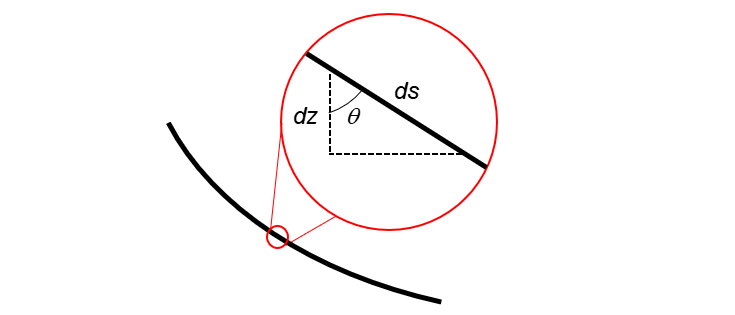
Fig. 1—Relationship between \(z\) and \(s\)
If we define the angle \(\theta\) as the deviation from vertical (often referred to as inclination), we can obtain the following relationship Hence, the gravity pressure gradient in \eqref{grav_grad_one} become
Friction Pressure Gradient
The friction pressure gradient for pipe flow is described by the Darcy-Weisbach equation where \(\rho_f\) is the density used in the friction pressure gradient.
Acceleration Pressure Gradient
The acceleration pressure gradient for pipe flow is expressed as where \(\rho_a\) is the density used in the acceleration pressure gradient. The appendix in Beggs and Brill (1973)3 gives a detailed walkthrough of how the acceleration pressure gradient can be simplified to eliminate the velocity derivative. The resulting expression is We see that the acceleration pressure gradient is a function of the total pressure gradient.
Total Pressure Gradient
Adding together the expressions for gravity-, friction-, and acceleration pressure drops, we get the following expression for the pressure drop in the well which is rewritten to the final expression for the pressure gradient As many of the properties in \eqref{pres_grad} is pressure- and temperature depedendent, \eqref{pres_grad} is a nonlinear, first-order, ordinary differential equation that needs to be solved numerically. This can be done explicitly (forward marching) by using for example a Runge-Kutta method, or it can be solved implicitly as a system of equations.
Temperature Profile
The temperature profile in the well can be estimated in many ways. The simplest would be to assume the temperature equal to the surrounding rock temperature, but this is not be a very good approximation. In fact, that assumption implies that the fluid cools infinitely fast, which is unphysical. A different approach is to model the temperature loss from inlet to outlet using some average properties to describe the heat loss. The following equation is based on simple thermodynamic relations
where \(K=U/c_p\) is a constant one often have to solve for. The rock temperature is often assumed to be linear with vertical depth, meaning it can be expressed as
where \(T_R\) is the reservoir temperature, and \(\alpha=(T_R-T_{surf})/(z_R-z_{surf})\). Inserting \eqref{rock_temp} into \eqref{temp_grad_one} and rearranging yields
which is a first-order, linear ODE on the form \(y'+p(x)y=q(x)\) having a general solution Solving \eqref{gen_form} by applying \eqref{gen_sol} results in The initial condition \(T(0)=T_R\) yields the integration constant \(C=-\alpha\cos(\theta)\dot{m}/(K\pi d_h)\), and so the final expression for the temperature profile is The unknown in this equation is \(K\), which can be solved for numerically by knowledge of the temperature somewhere along the length of the pipe. For flow in wells, it is common to use the wellhead temperature (i.e. the flow temperature at the pipe outlet) to estimate \(K\).
-
N. Zuber and J. A. Findlay. Average Volumetric Concentration in Two-Phase Flow Systems. Journal of Heat Transfer, 87:453–468, 11 1965. doi:10.1115/1.3689137. ↩
-
L.F. Moody. Friction Factors for Pipe Flow. Transactions of the ASME, 66:671–684, 1944. ↩
-
H.D. Beggs and J.P. Brill. A study of two-phase flow in inclined pipes. Journal of Petroleum Technology, pages 607–617, 5 1973. SPE-4007-PA. doi:10.2118/4007-PA. ↩