Binary Interaction Parameters

The binary interaction parameters (BIPs) are a set of correction terms to the mixing rule for the model parameter "$a$" in the cubic equation of state models. The BIPs were introduced by Chueh and Prausnitz in 1967¹ and has been shown to have a major impact on phase behavior calculations. The introduction of the BIPs into the mixing rule are given below and typically range from -0.1 to 0.2, but are physically bounded by -1 to 1. As a rule of thumb, the BIPs should increase with increasing with increasing separation of components (e.g. the BIP between $C_1$ and $C_{30}$ should be larger than the BIP between $C_1$ and $C_{29}$).

whitson comment

Note from Markus Hays Nielsen: Negative BIPs, although physical, have a tendency to create non-physical extrapolations of the K-value data (low and/or high pressures). We therefore recommend caution if you choose to apply negative BIPs in your EOS model.

Methods for choosing a value for the BIPs range from a wide range of correlations, to tuning, to a combination of both correlations and tuning. These three different approaches are discussed in the following sections for some correlations and methods for tuning. It is worth noting that the aim of introducing BIPs is, in some ways, to avoid having to introduce different or more complex mixing rules.

Several authors have noted that the magnitude of the BIPs in different equation of state models differ. Typically, the magnitude of the Soave-Redlich-Kwong (SRK) EOS model tend to be smaller than those of the Peng-Robinson (PR) EOS model. This has led some to assume that the BIPs are of less importance for the SRK EOS and can therfore be ignored (set to zero) for hydrocarbon-hydrocarbon components². This holds for some fluid systems, but it has been shown that even for the SRK EOS model, BIPs can significantly improve the fit of the model to PVT data³.

Correlations

Chueh-Prausnitz Correlation

The first BIP correlation was developed by Chueh and Prausnitz¹ and is given by

$\begin{equation}\label{eq:chueh_prausnitz} k_{ij} = 1 - (\frac{\sqrt{v_{ci}^{1/3}v_{cj}^{1/3}}}{(v_{ci}^{1/3}+v_{cj}^{1/3})/2})^n \end{equation}$

where $n$ is an empirical parameter that can be adjusted for a given fluid system.

Gao Correlation

A correlation was proposed by Gao in 1992⁴ for the PR EOS, given by

$\begin{equation}\label{eq:gao} k_{ij} = 1 - (\frac{2 \cdot \sqrt{T_{ci}T_{cj}}}{T_{ci}+T_{cj}})^{\frac{Z_{ci}+Z_{cj}}{2}} \end{equation}$

where $T_{ci}$ is the component critical temperature, and $Z_{ci}$ is the component critical Z-factor.

Coutinho et al. Correlation

Another correlation was developed by Countinho in 1994⁵ for the SRK EOS, given by

$\begin{equation}\label{eq:coutinho} k_{ij} = 1 - A(\frac{\sqrt{b_ib_j}}{b_{ij}})^\theta \end{equation}$

where

$\begin{equation}\label{eq:bij_def} b_{ij} = \frac{1}{8}(b_i^{1/3}+b_j^{1/3})^3 \end{equation}$

In equation \eqref{eq:coutinho} $A$ and $\theta$ are empirical parameters that can be adjusted for a given fluid system.

Group Contribution Correlation

Note

For this correlation the temperature is assumed to be in Kelvin.

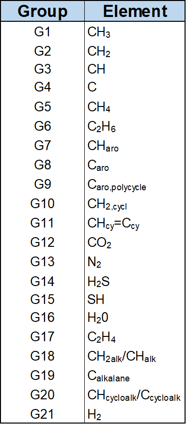
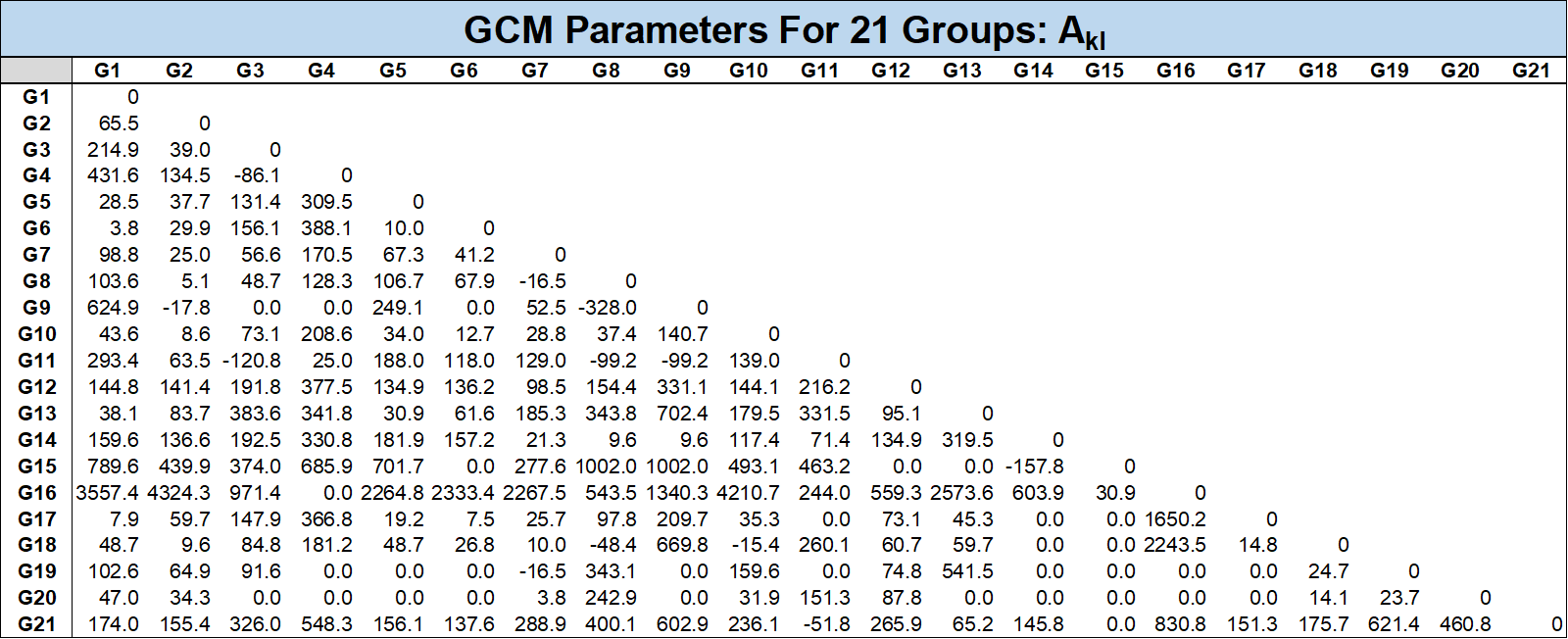
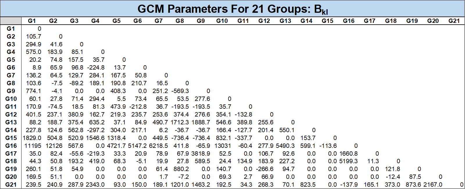
A semi-analytical model was developed by Jaubert et al. after 2004⁶ based on a group contribution method. The approach for isomers is given below

$\begin{equation}\label{eq:GCM} k_{ij} = \frac{-1/2\sum_{k=1}^{N_g}\sum_{l=1}^{N_g}(\alpha_{ik}-\alpha_{jk})(\alpha_{il}-\alpha_{jl}) A_{kl}\cdot (298.15/T)^{(\frac{B_{kl}}{A_{kl}}-1)}-(\frac{\sqrt{a_i(T)}}{b_i}-\frac{\sqrt{a_j(T)}}{b_j}) }{2\frac{\sqrt{a_i(T)a_j(T) }}{b_ib_j}} \end{equation}$

where $a_{ik}$ is the fraction of elements in group $i$ for component $k$ and the constants $A_{kl}$ and $B_{kl}$ are the universal group interaction parameters. The list of all groups and their corresponding $\alpha$ fractions and group interaction parameters are given in the tables below.

Table 1: List of all groups in Jaubert et al. GCM BIP correlation.

Jaubert group comtribution bips parameters

Table 2: Constant $A_kl$ values for the 21 groups given in Table 1.

Table 3: Constant $B_kl$ values for the 21 groups given in Table 1.

There is also an approach proposed by Jaubert et al. to estimate BIPs for pseudo-components using a PNA correlation based on the $T_c$, $p_c$ and $\omega$ for the component. This approach splits the pseudo-component into several parafinic, aromatic and maphthanic groups based on the component properties.

Tuning

In general, tuning BIPs should be treated with caution as there are numerous adjustments that can give non-physical phase behavior. One key metric used to check for physical consistency is K-value crossing between HC-HC component K-values. The reason why crossing K-values are assumed to be non-physical is because this would indicate that a heavier component would prefere to be in the lighter phase more than a lighter component and this goes against the evidence for hydrocarbon systems. Since the 1960's when Chueh and Prausnitz published on the topic of BIPs, several correlations and work-flows have been proposed. In the following sections, some of these workflows are highlighted, but a note of caution is also granted for all these methods as there is little to no consensus in the literature of the "correct" approach. This is made evident by the fact that none of the major PVT software's have a consistent BIP tuning module.

Katz-Firoozabadi Approach

In 1978 Katz and Firoozabadi published an approach to BIP tuning that they had found to be effective for a number of real HC fluid systems⁷. The empirical results showed that tuning of the BIP between the lightest HC and the heavy $C_{n+}$ fraction gives a consistently better phase behavior prediction.

This approach has become a standard rule of thumb for EOS modeling. When testing different correlations (e.g. Chueh-Prausnitz, Coutinho et al. and GCM) the general trend indicates that there is an increasing value for the BIP with increasing difference in the HC size (i.e. molecular weight or true boiling point). Several of the correlations for the BIPs refer to semi-analytic derivations of the BIP correlation, which indicate (indirectly) that this feature is inherent in the behavior of BIPs.

Mixed Correlation Approach (Younus et al.)

In a comprehensive paper on the development of field-wide EOS models, Younus et al. describe a process for tuning the BIPs⁸. The approach described, and applied by us at whitson, is a combination of (1) first applying the Chueh-Prausnitz (as this is implemented in PhazeComp) between the light components and the heaviest fractions with a scaling multiplier, then (2) adjust single BIPs to try and improve the match of the PVT-data. This mixed correlation and tuning approach is possible and effective because of the degree of knowledge built at whitson over 30 years.

Gani-Fredenslund Approach

In a paper from 1987, Gani and Fredenslund describe an approach for EOS model development with BIPs (called expert tuning) by determining the most important adjustable parameters³. Their method determines (1) if EOS model tuning is recommended and (2) if tuning is recommended, then what tuning approach is recommended for the type of PVT data available.

For the second point, their tuning approach is divided into two parts: (a) adjusting the volume shifts or (b) tune the components properties or BIPs depending on their metric for the most important adjustable variable. Gani and Fredenslund also divide the modeling type and fluid mixture type based on the available data (e.g. compressibility or a full CCE test) and which component properties are determined to have the greatest impact on the tuning.

The proposed approach by Gani and Fredenslund has not gained wide spread acceptance, but is a unique attempt to do consistent EOS modeling with BIPs.

Other Tuning Approaches

Other authors have independently re-discovered the main idea of Gani and Fredenslund like Liu in 1999⁹ with his "fully automatic procedure for efficient reservoir fluid characterization" and Nielsen in 2020 (MSc Thesis) with his "selctive tuning" approach. Both authors use derivarive based methods to determine the importance of different tunable parameters of the EOS model.

P.L. Chueh and J.M. Prausnitz. Vapor-liquid equilibria at high pressures: calculation of partial molar volumes in nonpolar liquid mixtures. AIChE journal, 13:1099–1107, 1967. doi:https://doi.org/10.1002/aic.690130612. ↩↩
K.S. Pedersen, P. Thomassen, and Aa. Fredenslund. On the dangers of tuning equation of state parameters. Tuning” equation of state parameter,” Society of Petroleum Engineers of AIME, pages 14487, 1985. doi:https://doi.org/10.1016/0009-2509 $88$ 85039-5. ↩
R. Gani and Aa. Fredenslund. Thermodynamics of petroleum mixtures containing heavy hydrocarbons: an expert tuning system. Industrial & engineering chemistry research, 26:1304–1312, 1987. doi:https://doi.org/10.1021/ie00067a008. ↩↩
Guanghua Gao, Jean-Luc Daridon, Henri Saint-Guirons, Pierre Xans, and François Montel. A simple correlation to evaluate binary interaction parameters of the peng-robinson equation of state: binary light hydrocarbon systems. Fluid phase equilibria, 74:85–93, 1992. ↩
João AP Coutinho, Georgios M Kontogeorgis, and Erling H Stenby. Binary interaction parameters for nonpolar systems with cubic equations of state: a theoretical approach 1. co2/hydrocarbons using srk equation of state. Fluid phase equilibria, 102:31–60, 1994. ↩
J.N. Jaubert and F. Mutelet. Vle predictions with the peng–robinson equation of state and temperature dependent kij calculated through a group contribution method. Fluid Phase Equilibria, 224:285–304, 2004. doi:https://doi.org/10.1016/j.fluid.2004.06.059. ↩
D. L. Katz and A. Firoozabadi. Predicting phase behavior of condensate/crude-oil systems using methane interaction coefficients. Journal of Petroleum Technology, 30:paper SPE–6721–PA, 1978. doi:https://doi.org/10.2118/6721-PA. ↩
B. Younus*, C. H. Whitson, A. Alavian, M. L. Carlsen, S. Martinsen, and K. Singh. Field-wide equation of state model development. In Unconventional Resources Technology Conference, Denver, Colorado, 22-24 July 2019, paper URTeC551. Unconventional Resources Technology Conference $URTeC$ ; Society of …, 2019. doi:https://doi.org/10.15530/urtec-2019-551. ↩
K. Liu. Fully automatic procedure for efficient reservoir fluid characterization. In SPE Annual Technical Conference and Exhibition, paper SPE–56744–MS. Society of Petroleum Engineers, 1999. ↩