Cubic Equation of State Models

A cubic equation of state (EOS) is a fluid model that describes relationship between the variables pressure, temperature, volume and composition (see PVT for more info). The reason for the name "cubic" is because of the cubic polynomial approximation used to approximate the Z-factor or equivalently the molar volume. This is shown in equation \eqref{eq:ceos}. Some common cubic equation of state models are the van der Waals (vdW) EOS¹, Peng-Robinson (PR) EOS² and Soave's modification to the Redlich-Kwong EOS (SRK)³. Unlike other multi-phase EOS models like the Benedict-Webb-Ruben (BWR)⁴ and higher order virial EOS models, the cubic EOS models can be generalized by

$\begin{equation}\label{eq:ceos} A_0 + A_1\cdot Z +A_2\cdot Z^2 + A_3\cdot Z^3 = 0 \end{equation}$

where $A_0$, $A_1$, $A_2$ and $A_3$ are constants determined by the particular EOS model.

Historical Overview

The first cubic EOS was developed in 1873 by Johannes van der Waals as part of his Ph.D. dissertation¹ for which he was awarded with a Nobel price in physics. The EOS was able to model the phase behavior of vapor and liquids more accurately than any other existing model. The vdW EOS has since derived from kinematic theory based on statistical mechanics.

The first cubic EOS model developed for the use in petroleum industry was developed by Redlich and Kwong in 1949⁵ that was modified by Soave in 1972³. Following the SRK EOS, another cubic EOS was developed in 1976 by Peng and Robinson ⁶ which was modified in 1978 by Peng and Robinson². The SRK and the 1978 PR EOS are the most common EOS models used in petroleum and chemical engineering to this day and are used as standard models in most PVT packages.

Structure of a Cubic EOS

As shown in equation \eqref{eq:ceos}, a cubic EOS is defined by a cubic polynomial equation with repect to either the Z-factor or volume (typically the molar volume). However, a more common general description of the cubic EOS models can be written as

$\begin{equation}\label{eq:ceos_general} p = \frac{RT}{v-b} - \frac{a}{D(v)} \end{equation}$

where $a$ and $b$ are the EOS model parameters and $D(v)$ is a 2nd degree polynomial with respect to the molar volume $v$. Some examples of $D(v)$ for the previously mentioned EOS models are given by

EOS Model	Denominator: $D(v)$
van der Waals	$v^2$
Peng-Robinson	$v(v+b)+b(v-b)$
Soave-Redlich-Kwong	$v(v+b)$

To have a consistent and useful EOS model for multi-component fluid systems, the EOS parameters $a$ and $b$ must be defined from the known components properties and a set of mixing rules.

Component Properties

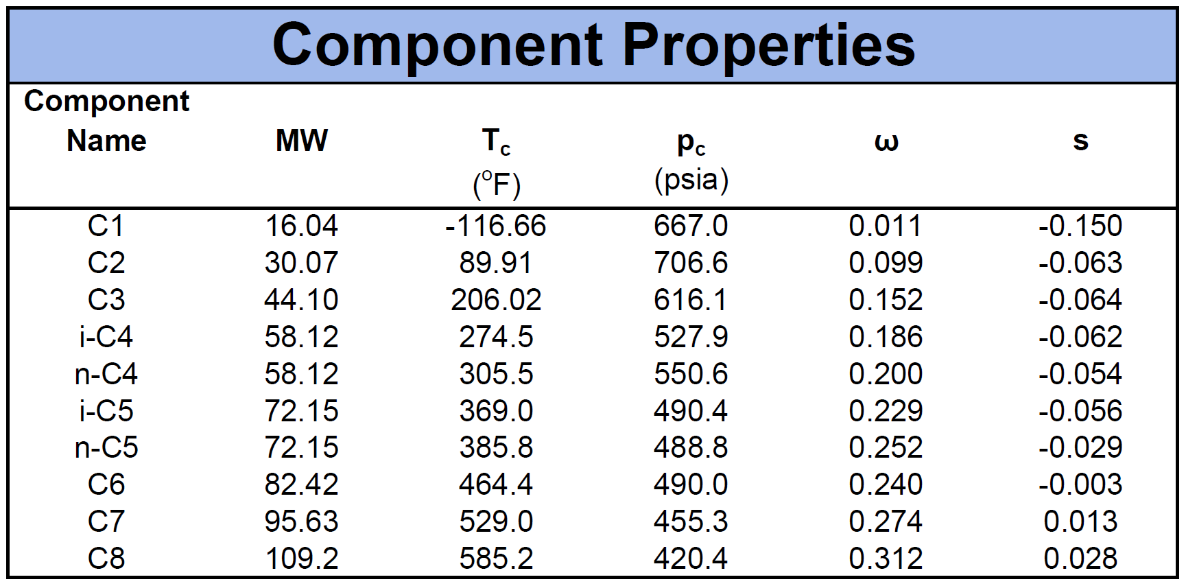
The component properties are composed of the critical pressure ($p_c$), critical temperature ($T_c$), acentric factor ($\omega$) and molecular weight ($MW$). Another important component property for cubic EOS models is the volume shift factor descried by Peneloux in 1982⁷. The volume shifts were introduced as a correction term to the phase behaviour predictions of the molar volume curve. An example of a fluid mixture's component properties is given by

Table 1: Example of EOS component properties for a multi-component fluid mixture.

Mixing Rules

The original mixing rule developed by van der Waals is a quadratic mixing rule. The set of equations describing the mixing are given by

$\begin{equation}\label{eq:a_mix_vdw} a = \sum_{i=1}^N \sum_{i=1}^N u_i u_j a_{ij} \end{equation}$

$\begin{equation}\label{eq:b_mix_vdw} b = \sum_{i=1}^N u_i b_i \end{equation}$

where $a_{ij}=\sqrt{a_ia_j}$, $u_i$ can be the liquid composition ($x_i$), vapor composition ($y_i$) or the total composition ($z_i$) and $a_i$ and $b_i$ are the component EOS parameters for component $i$. These mixing rules are often refered to as the van der Waals mixing rules.

The quadratic mixing rules are typically used and on of the most convincing arguments for using this type of mixing rule is that it satisfies the compositional dependency of the second virial coefficient.

Modifications to the $a$ and $b$ mixing rules were developed to enhance the performance of the EOS models. The most common modified mixing rules are given by

$\begin{equation}\label{eq:a_mix_mod} a = \sum_{i=1}^N \sum_{i=1}^N u_i u_j a_{ij} (1-k_{ij}) \end{equation}$

$\begin{equation}\label{eq:b_mix_mod} b = \sum_{i=1}^N u_i b_i(1-l_{ij}) \end{equation}$

whitson comment

Note from Markus Hays Nielsen: Even though we have given the correction term for the mixing rule of the b-parameter, we do not recommend using values of $l_{ij}$ other than zero. There are several reasons for this, but one major reason is that most PVT software does not allow for these parameters to be input.

where $k_{ij}$ and $l_{ij}$ are the corrections parameters. The first application of these correction parameters for the b-parameter was published by Yarborough⁸. It is common to neglect the correction parameter for the mixing rule of $b$ and only consider the correction parameter for $a$. The remaining correction parameter ($k_{ij}$) is often referred to as the binary interaction parameter (BIP) or sometimes referred to as the binary interaction coefficient (BIC). Because there is a separate BIP between each component pair, the number of BIPs will be defined by

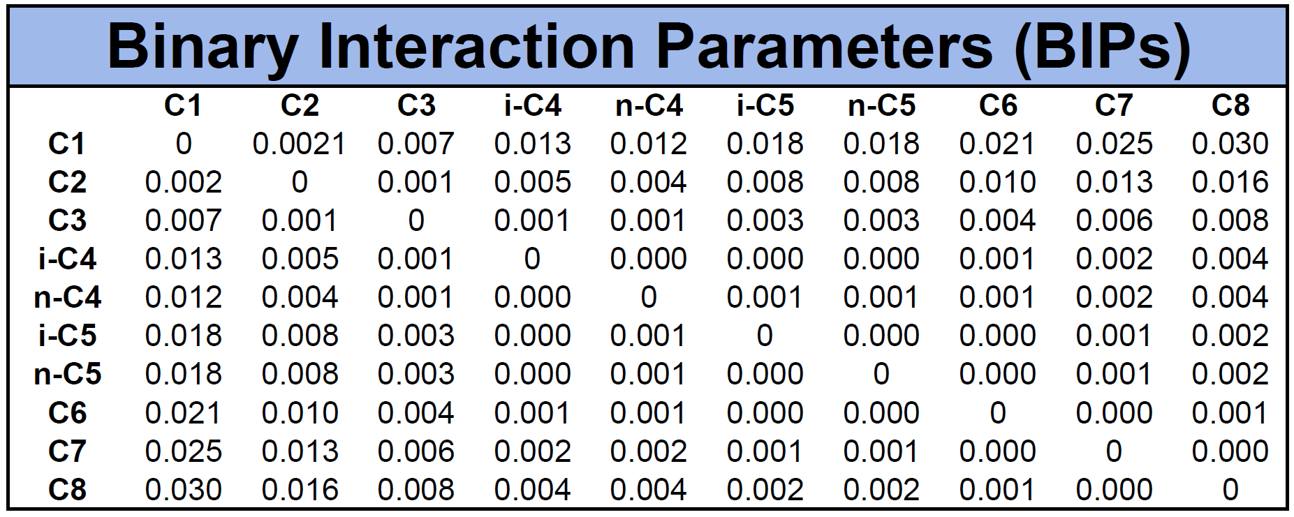
$\begin{equation}\label{eq:bips_comps_number} N_{bips} = \frac{N_{comps}\cdot (N_{comps}-1)}{2} \end{equation}$

The BIPs can be defined by a correlation like the Cheuh-Prausnitz correlation ⁹ or the group contribution correlation correlation by Jaubert et al¹⁰, or the BIPs can be tuned to phase behavior data for specific subsets of BIPs like Katz and Firoozabadi showed was effective in 1978¹¹.

An example of BIPs for the mixture given in Table 1 is given in Table 2 based on the Chueh-Prausnitz correlation without tuned model coefficients.

Table 2: Example of BIPs for the multi-component fluid mixture given in Table 1.

Other mixing rules like the one by Smith et al.¹², Pesuit et al.¹³, etc. have also shown to be effective for some cases, but have not gained wide spread use in the industry.

Other Cubic EOS Models

There are a wide range of other cubic EOS models. These models typically modify the original approach by PR and RK. Modifications of the RK EOS include Soave's modification (SRK) as described above, but also different modification such as a modification by Zudkevitch and Joffe (ZJRK) who introduced temperature dependent correction terms for both EOS constants $a$ and $b$, also both being functions of acentric factor. Modifications were also made to the PR EOS, first by Peng and Robinson, then by Usdin and McAuliffe and Fuller. Martin has a detailed review of the different cubic EOS models and introduces his own variation¹⁴. His comment on which EOS model is best, he cites Snow White: "mirror mirror on the wall, who's the fairest of them all". This statement reflects the current state of EOS modeling just as well as when he wrote his summary in 1979.

J.D. Van der Waals. On the continuity of the gaseous and liquid states. Universiteit Leiden, 1873. ↩↩
D. B. Robinson and D. Y. Peng. The characterization of the heptanes and heavier fractions for the GPA Peng-Robinson programs. Gas processors association, 1978. ↩↩
G. Soave. Equilibrium constants from a modified redlich-kwong equation of state. Chemical engineering science, 27:1197–1203, 1972. doi:https://doi.org/10.1016/0009-2509 $72$ 80096-4. ↩↩
M. Benedict, G. B. Webb, and L. C. Rubin. An empirical equation for thermodynamic properties of light hydrocarbons and their mixtures i. methane, ethane, propane and n-butane. The Journal of Chemical Physics, 8:334–345, 1940. doi:https://doi.org/10.1063/1.1750658. ↩
O. Redlich and J. N. S. Kwong. On the thermodynamics of solutions. v. an equation of state. fugacities of gaseous solutions. Chemical reviews, 44:233–244, 1949. ↩
D. Y. Peng and D. B. Robinson. A new two-constant equation of state. Industrial & Engineering Chemistry Fundamentals, 15:59–64, 1976. ↩
A. Péneloux, E. Rauzy, and R. Fréze. A consistent correction for redlich-kwong-soave volumes. Fluid phase equilibria, 8:7–23, 1982. doi:https://doi.org/10.1016/0378-3812 $82$ 80002-2. ↩
L. Yarborough. Application of a generalized equation of state to petroleum reservoir fluids. ACS Publications, 1979. ↩
P.L. Chueh and J.M. Prausnitz. Vapor-liquid equilibria at high pressures: calculation of partial molar volumes in nonpolar liquid mixtures. AIChE journal, 13:1099–1107, 1967. doi:https://doi.org/10.1002/aic.690130612. ↩
J.N. Jaubert and F. Mutelet. Vle predictions with the peng–robinson equation of state and temperature dependent kij calculated through a group contribution method. Fluid Phase Equilibria, 224:285–304, 2004. doi:https://doi.org/10.1016/j.fluid.2004.06.059. ↩
D. L. Katz and A. Firoozabadi. Predicting phase behavior of condensate/crude-oil systems using methane interaction coefficients. Journal of Petroleum Technology, 30:paper SPE–6721–PA, 1978. doi:https://doi.org/10.2118/6721-PA. ↩
W. R. Smith. Perturbation theory and one-fluid corresponding states theories for fluid mixtures. The Canadian Journal of Chemical Engineering, 50:271–274, 1972. doi:https://doi.org/10.1002/cjce.5450500223. ↩
D. R. Pesult. Binary interaction constants for mixtures with a wide range in component properties. Industrial & Engineering Chemistry Fundamentals, 17:235–242, 1978. ↩
J. J. Martin. Cubic equations of state-which? Industrial & Engineering Chemistry Fundamentals, 18:81–97, 1979. ↩

EOS Model	Denominator: \(D(v)\)
van der Waals	\(v^2\)
Peng-Robinson	\(v(v+b)+b(v-b)\)
Soave-Redlich-Kwong	\(v(v+b)\)