Beggs and Brill

General Description

The correlation for two-phase flow by Beggs and Brill (1973)¹ is based on experimental work on a total of 584 experiments with the following ranges of variation

Gas Flow Rate: 0 to 300 Mscf/D
Liquid Flow Rate: 0 to 30 gal/min
Average System Pressure: 35 to 95 psia
Pipe Diameter: 1 and 1.5 in
Liquid Hold Up: 0 to 0.870
Pressure Gradient: 0 to 0.800 psi/ft
Inclination Angle: -90° to +90°
Fluids: Air and Water

The correlation relies on estimating the liquid hold up for horizontal flow from the predicted flow regime. The liquid hold up is then corrected for inclination by applying a correction factor $\psi$

$\begin{equation} \frac{H_L(\phi)}{H_L(0)}=\psi \end{equation}$ where $\phi$ is the angle from horizontal, which is connected to inclination by $\phi=\pi/2-\theta$.

The flow regime was suggested to be predicted by the use of a log-log plot of the liquid-flux fraction $C_L$ versus the dimensionless Froude number $N_{Fr} = v_m^2/(gd_h)$. The original publication contained a flow-regime map as shown in Fig. 1 (top), which was later updated² to the map shown in Fig. 1 (bottom).

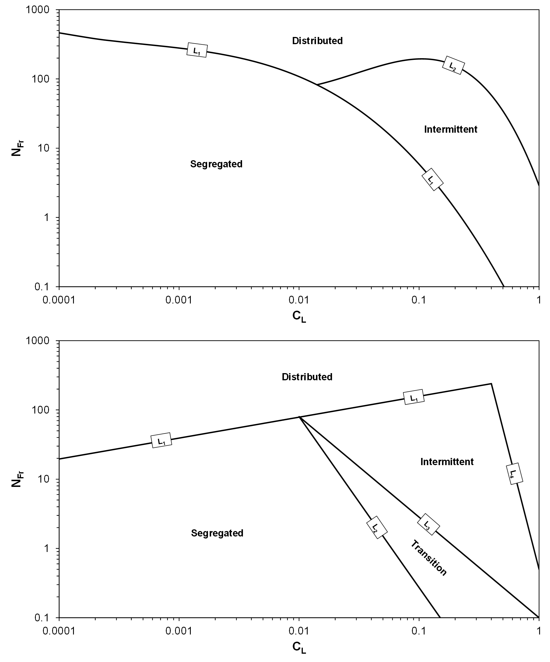
Fig. 1—Flow-regime maps. Top: Flow map from original publication. Bottom: Updated flow map.

The flow-regime boundaries in the top plot are calculated by

$\begin{align} &L_1=\exp(-4.62-3.757X-0.481X^2-0.0207X^3)\\ &L_2=\exp(1.061-4.602X-1.609X^2-0.179X^3+0.635\times 10^{-3}X^5) \end{align}$

where $X=\ln(C_L)$. For the bottom plot, the boundaries are calculated by

$\begin{align} &L_1=316C_L^{0.302}\\ \label{l1} &L_2=9.252\times 10^{-4}C_L^{-2.468}\\ &L_3=0.1 C_L^{-1.4516}\\ &L_4=0.5 C_L^{-6.738} \label{l4} \end{align}$

The flow regime intepretation for the updated flow map is as follows:

Segregated

$\begin{align} C_L < 0.01\quad&\text{and}\quad N_{Fr}\leq L_1,\text{ or}\\ 0.01\leq C_L\quad&\text{and}\quad N_{Fr}\leq L_2 \end{align}$

Intermittent

$\begin{align} 0.01\leq C_L < 0.4 \quad&\text{and}\quad L_3<N_{Fr}\leq L_1,\text{ or}\\ 0.4\leq C_L\quad&\text{and}\quad L_3\leq N_{Fr}\leq L_4 \end{align}$

Distributed

$\begin{align} C_L < 0.4 \quad&\text{and}\quad L_1< N_{Fr},\text{ or}\\ 0.4\leq C_L\quad&\text{and}\quad L_4< N_{Fr} \end{align}$

Transition

$\begin{align} 0.01\leq C_L\quad&\text{and}\quad L_2<N_{Fr}<N_3 \end{align}$

Liquid Hold Up for Horizontal Flow

The horizontal-flow liquid hold up is estimated by the following equation $\begin{equation} H_L(0) = AC_L^{\alpha} N_{Fr}^{\beta} \end{equation}$ where the coefficient and exponents are summarized in Table 1.

Table 1—Coefficient and exponents for horizontal liquid hold up

Horizontal Flow Pattern	$A$	$\alpha$	$\beta$
Segregated	$0.98$	$0.4846$	$-0.0868$
Intermittent	$0.845$	$0.5351$	$-0.0173$
Distributed	$1.065$	$0.5824$	$-0.0609$

Liquid Hold for Inclined Flow

The correction for pipe inclination $\psi$ are calculated as $\begin{equation} \psi = 1+B\bigg(\sin(\phi)-\frac{1}{3}\sin^3(\phi)\bigg) \end{equation}$ where the coefficient $B$ is calculated by $\begin{equation} B=(1-C_L)\ln(D\lambda^{\delta}N_{Fr}^{\epsilon}N_{Lv}^{\zeta}) \end{equation}$ with coefficient and exponents given in Tables 2 and 3.

Table 2—Coefficient and exponents for inclination correction term (uphill flow)

Horizontal Flow Pattern	$D$	$\delta$	$\epsilon$	$\zeta$
Segregated	$0.011$	$-3.768$	$-1.614$	$3.539$
Intermittent	$2.96$	$0.305$	$0.0978$	$-0.4473$
Distributed	$1$	$0$	$0$	$0$

Table 3—Coefficient and exponents for inclination correction term (downhill flow)

Horizontal Flow Pattern	$D$	$\delta$	$\epsilon$	$\zeta$
Segregated/Intermittent/Distributed	$4.7$	$-0.3692$	$-0.5056$	$0.1244$

Liquid Hold Up for Transition Flow Regime

If the flow regime is predicted to be "Transition", then a weighted average of the "Intermittent"- and "Distributed" boundary solutions are used. In other words, the liquid hold up for the "Transition" flow regime is given by:

$\begin{equation} H_L^{trans.}(N_{Fr}) = \eta\cdot H_L^{segr.}(L_2) + (1-\eta)\cdot H_L^{inter.}(L_3) \end{equation}$ where $\eta = (L_3-N_{Fr})/(L_3-L_2)$. The liquid hold up at the boundaries are obtained by backcalculting the corresponding $C_L$ from the boundary equations \eqref{l1}–\eqref{l4}.

Two-Phase Friction Factor

The Darcy friction $f_D$ is modified to account for two-phase effects. The modification suggested is $\begin{equation} \frac{f_{s}}{f_D}=\exp(S) \end{equation}$ where $f_s$ indicates friction factor for flow including slip. The exponent is given by $\begin{equation} S= \begin{cases} \ln(2.2y-1.2),&1.0<y<1.2\\ \frac{\ln(y)}{-0.0523+3.182\ln(y)-0.8725\ln(y)^2+0.01853\ln(y)^4}, &1.2\leq y \end{cases} \end{equation}$ where $y=C_L/(H_L(\phi))^2$.

Pressure Gradient Calculations

The correlation-specific properties in the pressure gradient are set to the following

Density in the gravity gradient $\rho_g=\rho_s$

Density in the friction gradient $\rho_f=\rho_m$

Density in the acceleration gradient $\rho_a=\rho_s$

Friction factor $f_D$ is calculated with $N_{Re}=\rho_m v_m d/\mu_m$

H.D. Beggs and J.P. Brill. A study of two-phase flow in inclined pipes. Journal of Petroleum Technology, pages 607–617, 5 1973. SPE-4007-PA. doi:10.2118/4007-PA. ↩
J.P Brill and D.H. Beggs. Two-Phase Flow in Pipes. Unknown Publisher, 6 edition, 1 1991. ↩

Horizontal Flow Pattern	\(A\)	\(\alpha\)	\(\beta\)
Segregated	\(0.98\)	\(0.4846\)	\(-0.0868\)
Intermittent	\(0.845\)	\(0.5351\)	\(-0.0173\)
Distributed	\(1.065\)	\(0.5824\)	\(-0.0609\)

Horizontal Flow Pattern	\(D\)	\(\delta\)	\(\epsilon\)	\(\zeta\)
Segregated	\(0.011\)	\(-3.768\)	\(-1.614\)	\(3.539\)
Intermittent	\(2.96\)	\(0.305\)	\(0.0978\)	\(-0.4473\)
Distributed	\(1\)	\(0\)	\(0\)	\(0\)