Equilibrium Ratios

The equilibrium ratio (K-value), defined in equation \eqref{eq:def}, is one of the most important thermodynamic quantities for petroleum systems. The reason for this is the direct connection it has on the flash calculation, which is a key phase behavior calculation. Furthermore, the K-values have an intuitive and simple physical meaning. Given a K-value for a specific component at certain conditions, the magnitude will determine the affinity the component has to be in the vapor phase (K-value greater than 1) or the liquid phase (K-value smaller than 1). Theoretically, the K-values can be measured in the lab and an argument can be made that accurate K-value measurements is the best source of PVT data used in equation of state model development.

The shape of the K-value is typically divided into the low-pressure region and the high-pressure region. For the low pressure region the K-values tend to be inversely proportional to the pressure (\(K_i \propto 1/p\)) yielding a -1 slope on a log-log plot and is said to follow Raoult's law and Dalton’s law

$$\begin{equation}\label{eq:raoult_dalton} K_i \approx \frac{p_{vi}(T)}{p} \end{equation}$$

where \(p_{vi}(T)\) is the vapor pressure of component \(i\). In the high-pressure region, all the K-values appear to converge to unity at the convergence pressure.

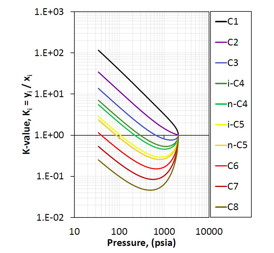
Figure 1: An example of pressure dependent K-values at a given temperature and composition.

Definition

The formal definition of the K-values are given by

$$\begin{equation}\label{eq:def} K_i = \frac{y_i}{x_i} \end{equation}$$

Areas of Use

The main area of use for the K-value is, as mentioned above, that it is a key quantity in the isothermal flash calculation. The K-value is some sense the driving mechanism behind most PVT calculations. The shape of the K-values (especially for high-pressures) drives the phase behavior of the fluid. For this reason, the K-value consistency check is essential as part of the equation of state model development.

Correlations

A wide range of correlations have been developed to estimate the K-values for hydrocarbon systems. However, as noted above, the only sure way to determine the true K-value is to solve the flash routine. Below, some correlations are given for reference.

Hoffman Correlation

$$\begin{equation}\label{eq:hoffman} K_i = \frac{10^{A_0+A_1F_i}}{p} \end{equation}$$

where

$$\begin{equation}\label{eq:Fi} F_i = \frac{1/T_{bi}-1/T}{1/T_{bi}-1/T_{ci}}\log{(p_{ci}/p_{sc})} \end{equation}$$

By re-arranging equation \eqref{eq:hoffman} and take the base-10 logarithm of both sides yield

$$\begin{equation}\label{eq:log_hoffman} \log{(K_ip)} = A_0+A_1F_i \end{equation}$$

such that \(A_0\) and \(A_1\) become the intercept and slope of a straight line on a log-log plot. This is the basis for the Hoffman quality check plot.

Wilson Correlation

$$\begin{equation}\label{eq:wilson} K_i = \frac{\exp{[5.37(1+\omega_i)(1-1/T_{ri})]}}{p_{ri}} \end{equation}$$

Note that the Wilson correlation is identical to the Hoffman correlation for \(A_0=\log{(p_{sc})}\) and \(A_1=1\) in equation \eqref{eq:hoffman} and the Edmister correlation ¹ is used for the acentric factor.

Modified Wilson Correlation

A modified version of the Wilson equation was proposed by Whitson and Torp in their 1981 paper ².

$$\begin{equation}\label{eq:mod_wilson} K_i = (\frac{p_{ci}}{p_k})^{A_1-1}\frac{\exp{[5.37\cdot A_1(1+\omega_i)(1-1/T_{ri})]}}{p_{ri}} \end{equation}$$

$$\begin{equation}\label{eq:A1} A_1 = 1-(p/p_k)^{A_2} \end{equation}$$

where \(A_2\) is a constant sometimes used defined as 0.7, \(p_{ci}\) is the component critical pressure, \(p_k\) is the convergence pressure, \(\omega_i\) is the acentric factor, \(p_{ri}\) is the reduced pressure defined by \(p_r=p/p_c\) and \(T_{ri}\) is the reduced temperature defined by \(T_r=T/T_c\). The units for equation \eqref{eq:mod_wilson} and \eqref{eq:A1} are psia for the pressure and R in temperature.

Standing Correlation

The Standing correlation for K-values was developed using the Hoffman correlation and tuned for low pressure K-value data³. The specified conditions where the correlation applies was described to be at \(p<1000\)psia and \(T<200^\circ\)F. The Standing correlation is often used to estimate the K-values for separator processes, specifically for the Hoffman plot quality check used for separator samples.

The equation for the Standing correlation is given by

$$\begin{equation}\label{eq:standing} K_i = \frac{10^{A_0+A_1F_i}}{p} \end{equation}$$

where

$$\begin{equation}\label{eq:Fi_standing} F_i = b_i(1/T_{bi}-1/T) \end{equation}$$

$$\begin{equation}\label{eq:bi_standing} b_i = \frac{\log{(p_{ci}/p_{sc})}}{1/T_{bi}-1/T_{ci}} \end{equation}$$

Unlike the Hoffman correlation, Standing gives an expression for \(A_0\) and \(A_1\) as a function of pressure. The correlation also gives a method for calculating \(b_i\) and \(T_{bi}\) for \(C_{7+}\) based on the pressure and temperature.

$$\begin{equation}\label{eq:A0_standing} A_0(p) = 1.2 + (4.5\cdot 10^{-4})p + (15\cdot 10^{-8})p^2 \end{equation}$$

$$\begin{equation}\label{eq:A1_standing} A_1(p) = 0.890 - (1.7\cdot 10^{-4})p - (3.5\cdot 10^{-8})p^2 \end{equation}$$

$$\begin{equation}\label{eq:bn_plus_standing} b_{n+} = 1013 + 324 n_{7+} - 4.256 n_{7+}^2 \end{equation}$$

$$\begin{equation}\label{eq:Tn_plus_standing} T_{b+} = 301 + 59.85 n_{7+} - 0.971 n_{7+}^2 \end{equation}$$

$$\begin{equation}\label{eq:n_plus} n_{7+} = 7.3 + 0.0075(T+459.67) + 0.0016p \end{equation}$$

In the Standing correlation given above, the units for pressure are in psia and the temperature is given in R.

Standing also gives a list of the component values for \(b_i\) and \(T_{bi}\) and they are given in the table below.

Component	\(b_i\)(cycle-\(^\circ\)R)	\(T_{bi}\) (\(^\circ\)R)
N\(_2\)	470	109
CO\(_2\)	652	194
H\(_2\)S	1136	331
C\(_1\)	300	94
C\(_2\)	1145	303
C\(_3\)	1799	416
i-C\(_4\)	2037	471
n-C\(_4\)	2153	491
i-C\(_5\)	2368	542
n-C\(_5\)	2480	557
C\(_6\)	2738	610

Simplified Flash

In 1986 Michelsen introduced a new approach to solve the flash in a simplified manner for an EOS model where all the BIPs were set to zero⁴. This simplified flash approach allows for a direct calculation of the K-values from the EOS parameters. The solution to Michelsen's procedure is given by

$$\begin{equation}\label{eq:simp_flash_coef} \ln{\phi_i} = q_0 + q_\alpha \alpha_i + q_\beta b_i \end{equation}$$

where \(b_i\) is the component EOS parameter and

$$\begin{equation}\label{eq:alpha} \alpha_i = a_{ii}^{0.5} \end{equation}$$

$$\begin{equation}\label{eq:q0} q_0 = -\ln{[\frac{p}{RT}(v-b)]} \end{equation}$$

$$\begin{equation}\label{eq:qa} q_\alpha = -\frac{2\alpha}{bRT(\delta_1-\delta_2)}\ln{(\frac{v+\delta_1b}{v+\delta_2b})} \end{equation}$$

$$\begin{equation}\label{eq:qb} q_\beta = \frac{1}{b}(\frac{pv}{RT}-1)+\frac{\alpha\cdot q_\alpha}{2b} \end{equation}$$

$$\begin{equation}\label{eq:alpha_mix} \alpha = \sum_{i=1}^Nu_i\alpha_i \end{equation}$$

where \(u_i\) can be the vapor molar amount (\(y_i\)) or liquid molar amount (\(x_i\)).

By using the fact that \(K_i = \phi_i^L/\phi_i^V\) and taking the natural logarithm of both sides yields

$$\begin{equation}\label{eq:simp_flash_correlation} \ln{K_i} = \ln{\phi_i^L} - \ln{\phi_i^V} \end{equation}$$

which can be calculated from equation \eqref{eq:simp_flash_coef}.

---

1. W. C. Edminster. Applied hydrocarbon thermodynamics, part 4: compressibility factors and equations of state. 1958. ↩

2. C. H. Whitson and S. B. Torp. Evaluating constant volume depletion data. In SPE Annual Technical Conference and Exhibition, paper SPE–10067–MS. Society of Petroleum Engineers, 1981. doi:https://doi.org/10.2118/10067-MS. ↩

3. M.B. Standing. A set of equations for computing equilibrium ratios of a crude oil/natural gas system at pressures below 1,000 psia. Journal of Petroleum Technology, 31:paper SPE–7903–PA, 1979. doi:https://doi.org/10.2118/7903-PA. ↩

4. M. L. Michelsen. Simplified flash calculations for cubic equations of state. Industrial & Engineering Chemistry Process Design and Development, 25:184–188, 1986. ↩